Ricker model

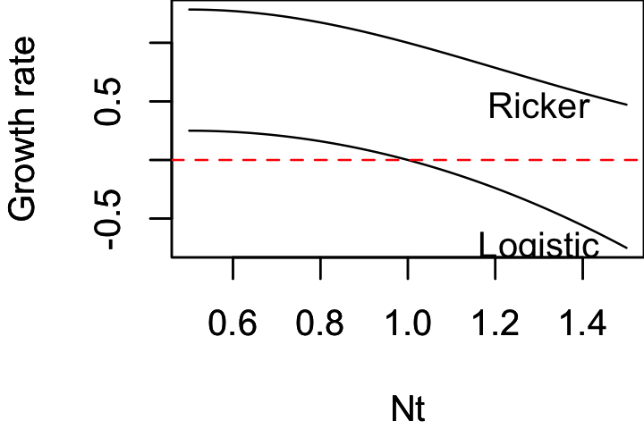
離散時間モデルの一つ
´ \[ N_{t+1} = \exp[r(1-\frac{N_t}{K})]N_t \]

Nが個体数、rが増殖率、Kが環境収容力

離散ロジスティックモデルとの違いは、 $ \exp $ をかけることで、増殖率が負にならないようにしている.

Code

# 環境収容力を１とした
logistic = \(Nt,r) r*(1-Nt/1)
ricker = \(Nt,r) exp( r*(1-Nt/1) )

df = data.frame(
    Nt = seq(0.5,1.5,0.01),
    r = seq(0.5,1.5,0.01),
    logistic = NA,
    ricker = NA
)
for(i in 1:nrow(df)){
    nt = df$Nt[i]
    r = df$r[i]
    df[i,"logistic"] = logistic(nt, r)
    df[i,"ricker"] = ricker(nt, r)
}

Code

xlim = range(df$Nt)
ylim = range(df[,3:4])
xlab = "Nt"
ylab = "Growth rate"

par(mar = c(4, 4, 0, 0)) 
plot(df$Nt, df[,"logistic"], type="l", 
     xlim=xlim, ylim=ylim,
     xlab=xlab, ylab=ylab)
par(new=TRUE)
plot(df$Nt, df[,"ricker"], type="l", 
     xlim=xlim, ylim=ylim,
     xlab=xlab, ylab=ylab)
abline(h=0, lty=2, col="red")

text(1.3, df[nrow(df),c("logistic")], "Logistic", cex=1)
text(1.3, df[nrow(df),c("ricker")], "Ricker", cex=1)

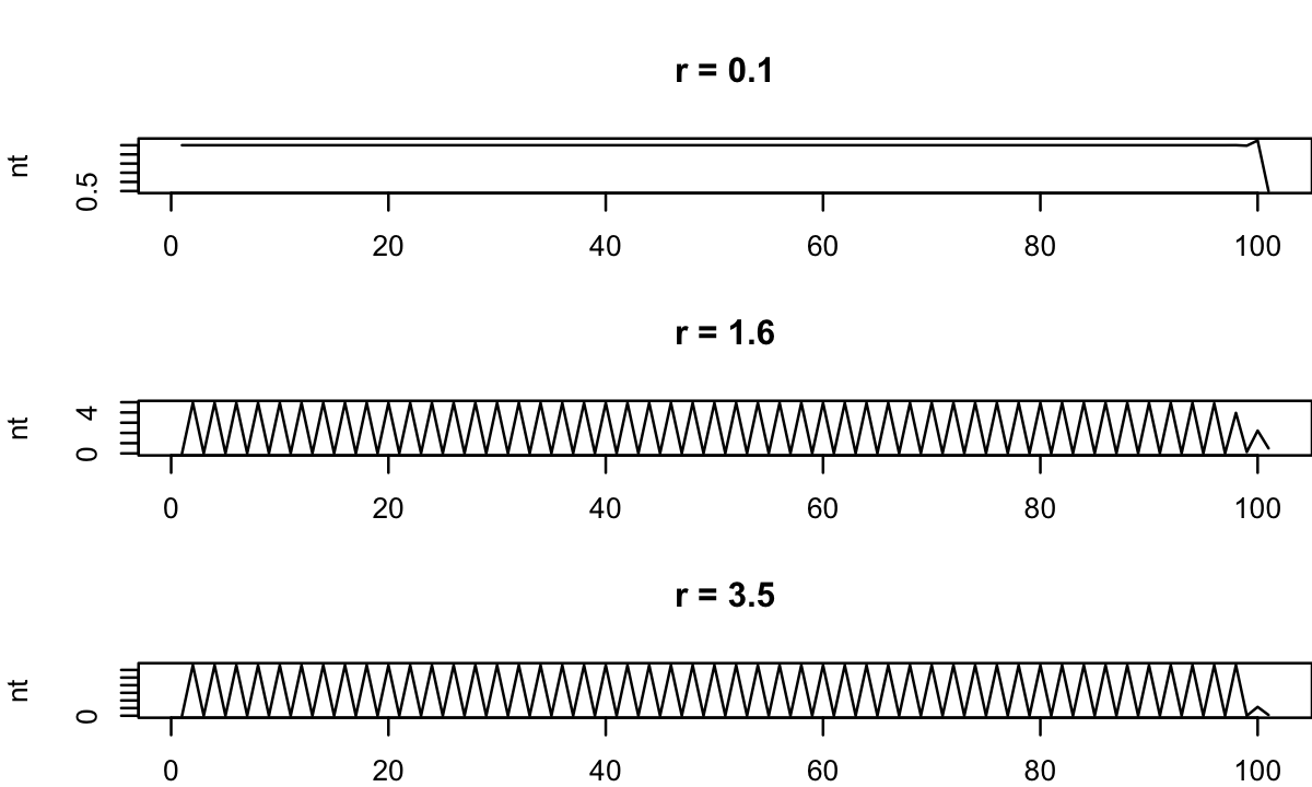
生態学においては、隣り合う世代が重なり合わない動態を記述する時に用いられるモデル. 観測データもそれにあたる？
例：１世代ごとに繁殖する虫, 観測データ

Code

par(
    mfrow =c (3,1),
    mar = c(2,4,4,0)
)

for(r in c(0.1, 1.6, 3.5)){

    nt = 0.5
    for(t in 1:100) nt = c(ricker(nt[1], r), nt)
    plot(nt, type='l', xlab="")
    title(paste("r =", r))
}

Code

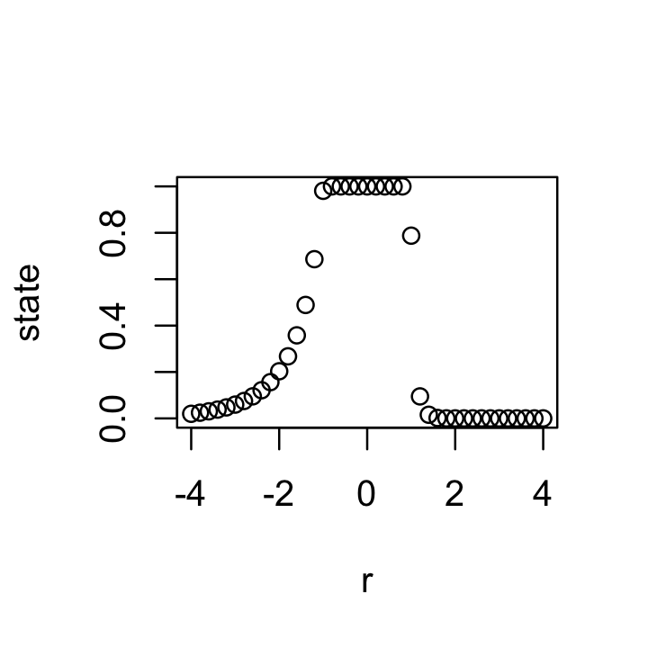
state = c()
for(r in seq(-4, 4, 0.2)){
    nt = 0.5
    for(t in 1:100) nt = ricker(nt, r)
    state = c(state, nt)
}

plot(seq(-4, 4, 0.2), state, xlab="r")

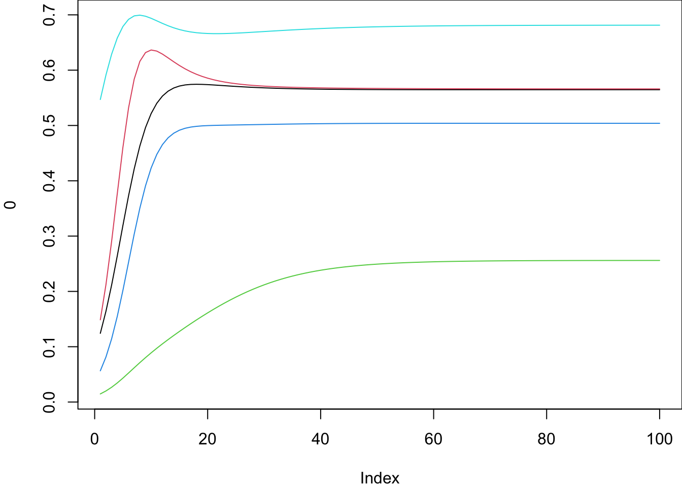
Multi-species Ricker model

\[ N_{i}(t+1) = \exp[r_i(1+e_iAN(t))]N_i(t) \] Nが個体数、rが増殖率、Kが環境収容力、M が相互作用行列、eが標準基底ベクトル（i番目=1、それ以外は0：i種が受ける影響をスカラーに直すためのもの）¹.

Code

set.seed(250721)

ms_ricker = \(N, r, A) exp( r*(1+A%*%N) ) * N

times = 100
sp = 10

# -- generate dynamics
N0 = as.integer( runif(sp, 1, 10) )
r = runif(sp, 0.2,0.5)

A = matrix(rnorm(sp*sp, mean=-0.2,sd=0.1), nrow=sp, ncol=sp)
A[which(abs(A)>0.25)] = 0
diag(A) = -1

mat = matrix(0, nrow=times, ncol=sp)
N = N0
for(i in 1:times) {N = ms_ricker(N, r, A); mat[i,]=N}
par(mar = c(4, 4, 0, 0)) 
plot(0, type="n", ylim=range(mat), xlim=c(1,times))
for(i in 1:5)lines(mat[,i], col=i)

Footnotes

Change et al., 2021, Ecol. lett.↩︎